> For the complete documentation index, see [llms.txt](https://help.connected.illumina.com/llms.txt). Markdown versions of documentation pages are available by appending `.md` to page URLs; this page is available as [Markdown](https://help.connected.illumina.com/dragen-stratamap/illumina-connected-multiomics/spatial-analysis/additional-analysis.md).

# Additional Analysis

[Filtering](#filtering)[ and Normalization](#filtering-and-normalization)

[PCA](#pca)

[UMAP](#umap)

[Clustering](#clustering)

[Differential Expression](#differential-expression)

[Marker Gene Identification](#marker-gene-identification)

[Cell Typing](#cell-typing)

[Cell-cell communication](#cell-cell-communication)

## Filtering and normalization

### Filtering

Filtering tasks offer flexibility to subsample your data for further downstream analyses. Filter data by:

* [Filter features](https://help.partek.illumina.com/partek-flow/user-manual/task-menu/filtering/filter-features)
* [Filter groups (samples or cells)](https://help.partek.illumina.com/partek-flow/user-manual/task-menu/filtering/filter-groups-samples-or-cells)
* [Filter barcodes](https://help.partek.illumina.com/partek-flow/user-manual/task-menu/filtering/filter-barcodes)
* [Split by attribute](https://github.com/illumina-swi/partek-docs/blob/main/docs/partek-flow/user-manual/task-menu/filtering/split-by-attributes.md)
* [Downsample cells](https://github.com/illumina-swi/partek-docs/blob/main/docs/partek-flow/user-manual/task-menu/filtering/downsample-cells.mds)

By default, the filtered counts node represents... from DRAGEN Spatial Transcriptome.

### Normalization and scaling

To ensure that data is comparable, several normalization and scaling options are available. Normalize or scale data by:

* [Impute low expression](https://github.com/illumina-swi/partek-docs/blob/main/docs/partek-flow/user-manual/task-menu/normalization-and-scaling/imput-low-expression.md)
* [Impute missing values](https://help.partek.illumina.com/partek-flow/user-manual/task-menu/normalization-and-scaling/impute-missing-values)
* [Normalization](https://help.partek.illumina.com/partek-flow/user-manual/task-menu/normalization-and-scaling/normalization)
* [Normalize to baseline](https://help.partek.illumina.com/partek-flow/user-manual/task-menu/normalization-and-scaling/normalize-to-baseline)
* [Normalize to housekeeping genes](https://help.partek.illumina.com/partek-flow/user-manual/task-menu/normalization-and-scaling/normalize-to-housekeeping-genes)
* [Scran deconvolution](https://help.partek.illumina.com/partek-flow/user-manual/task-menu/normalization-and-scaling/scran-deconvolution)
* [SCTransform](https://help.partek.illumina.com/partek-flow/user-manual/task-menu/normalization-and-scaling/sctransform)
* [TF-IDF normalization](https://help.partek.illumina.com/partek-flow/user-manual/task-menu/normalization-and-scaling/tf-idf-normalization)

By default, the normalization counts node represents ... from DRAGEN Spatial Transcriptome.

## PCA

Principal components (PC) analysis (PCA) is an exploratory technique that is used to describe the structure of high dimensional data by reducing its dimensionality. Therefore, the total variance of the original variables is equal to the total variance of the PCs. It is a principal axis rotation of the original variables that preserves the variation in the data. It is a linear transformation that converts n original variables into n new variables, which are called PCs, they have three important properties:

* PCs are ordered by the amount of variance explained
* PCs are uncorrelated
* PCs explain all variation in the data

### Invoke PCA task

PCA can be invoked from a counts node.

* Select a counts node on the canvas and then **PCA** in the *Exploratory analysis* section of the context sensitive menu
* Choose which features to include in the calculation
* Choose the number of PCs to calculate
* Choose how features should contribute
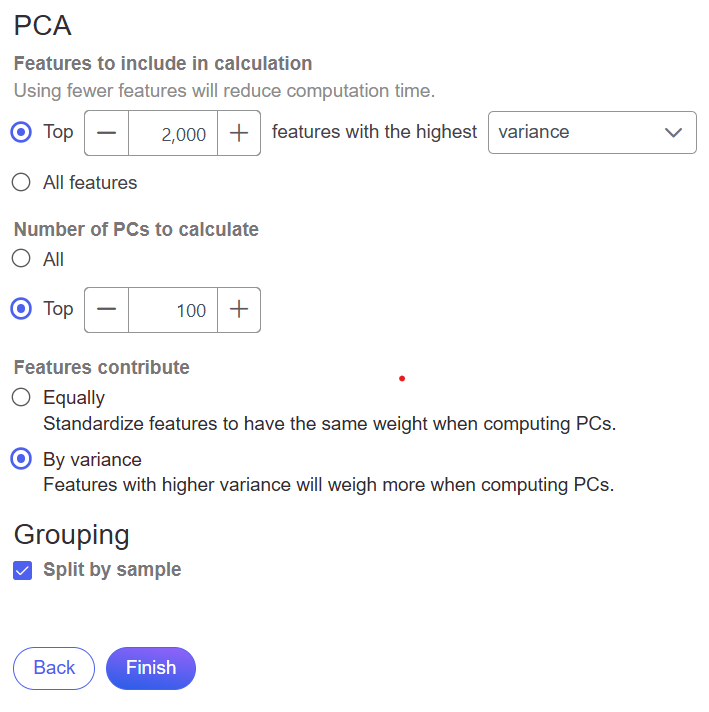
* If more than one sample is present in the project, choose to split by the sample or uncheck this option to group all samples together in the output

<figure><img src="/files/sRvseyWrodc8M19bXynB" alt=""><figcaption><p>Keep the default settings or adjust task settings accordingly</p></figcaption></figure>

### PCA task settings

There are options to include all features in the calculation or to reduce the number of features based on the argument stated.

* The default number of features to include are the Top 2000 features with highest variance

There are options for the number of PCs to calculate.

* The default number of PCs to calculate is the Top 100 PCs

There are two options for feature contribution:

* **equally**: all the features are standardized to mean of 0 and standard deviation of 1 . This option will give all the features equal weight in the analysis
* **by variance**: the analysis will give more emphasis to the features with higher variances. This is the default option for spatial counts

When more than one sample is present in the project, there is an option to split the samples (default) which will generate independent PCA results for each sample. If all samples should be including in one PCA results, uncheck this option.

### PCA outputs

The PCA task creates a new task node, and to open it and see the result, do one of the following:

* Select the PCA task node, proceed to the context sensitive menu and go to the Task result
* Double-click on the PCA task node

The default report is opened in the Data Viewer and contains:

* 3D scatterplot with the first three PCs shown on the X-, Y-, and Z-axis respectively, with the information content of an individual PC is in the parenthesis and each dot represents an observation
* Scree plot with Eigenvalues
* Component loadings matrix

As an exploratory tool, the the **PCA scatterplot** is applied to view any groupings in the data set and generate hypotheses based on the outcome, or to spot possible outliers.

* To rotate the 3D scatter plot left click & drag. To zoom in or out, use the mouse wheel. Click and drag the legend can move the legend to different location on the viewer.
* Use Axes to change the plotted PC
* Mouse over a point to display detailed information of the observation

The **Scree plot** with Eigenvalues shows how much variation each PC represents, so it is often used to determine the number of principal components to keep for downstream analysis (e.g. tSNE, UMAP, graph-base clustering). The "elbow" point of the graph where the Eigenvalues seem to level off should be considered as a cutoff point for downstream analysis.

* Mouse over on a point on the line to display detailed information of the PC

By default the table represents the **Components loadings matrix**. Component loadings are the correlation coefficients between the features and PCs. In the table, each row is a feature, the column represents PCs where the value is the correlation coefficient.

* The Content can be modified using Content (e.g. to change the content to PCA projections; in a PCA projections table each row is an observation, each column is a PC, and the values are PC scores)
* The table can be paged through within Content or from the lower right corner of the table

## UMAP

Uniform Manifold Approximation and Projection (UMAP) is a dimensional reduction technique \[1]. UMAP aims to preserve the essential high-dimensional structure and present it in a low-dimensional representation. UMAP is particularly useful for visually identifying groups in large high-dimensional data sets such as spatial data.

An alternative to UMAP is t-Distributed Stochastic Neighbor Embedding (t-SNE) \[2]. Both t-SNE and UMAP are useful for identifying similar groups in large high-dimensional data sets. A comparison of the techniques for visualizing single cell RNA-Seq data by the authors of UMAP suggests that UMAP runs faster, is more reproducible, gives a more meaningful organization of clusters, and preserves more information about the global structure of the data than t-SNE \[3].

### Invoke UMAP task

We recommend normalizing counts and running PCA prior to running UMAP, but the task will run on any counts data node. By default, the UMAP in the task graph has been run from a PCA data node.

* Click the counts data node
* Click the **Exploratory analysis** section of the toolbox
* Click **UMAP** (see task settings below for more information on parameters)
* Click **Finish** to run

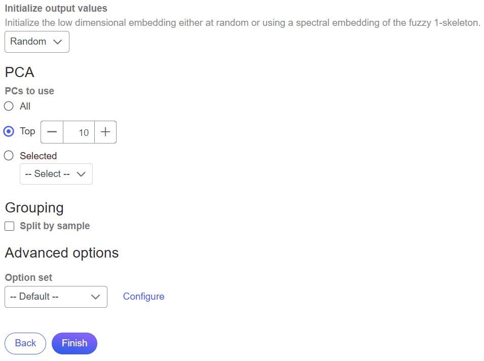
<figure><img src="/files/vF4HEEHkOzMN93t23pjx" alt=""><figcaption><p>Default UMAP task settings</p></figcaption></figure>

#### UMAP task settings

Initialize output values sets the initialization mode. Options are *Spectral* and *Random.*

* *Spectral* - good initial points are chosen using spectral embedding (more accurate)
* *Random* - random initial points are chosen (faster)

PCA is used to set the number of PCs to use or to specify a PC of interest by selecting this PC. By default, the top 10 PCs are used.

Grouping is used to split by sample and defaults to the setting used in the upstream data node. Chose whether to run UMAP on all samples together or on each sample individually if the upstream data node contains all samples. Checking the box will run UMAP on each sample individually.

For more information on [advanced UMAP parameters please refer to this documentation.](https://help.partek.illumina.com/partek-flow/user-manual/task-menu/exploratory-analysis/umap#advanced-umap-parameters)

### UMAP outputs

UMAP produces a UMAP task node. Opening the task report launches a scatter plot showing the UMAP results. Each point on the plot represents the spatial points. Hover an individual point to see more information about this point.

## Clustering

By default, Graph-based clustering is the method used to cluster and identify similar points. It makes no prior assumptions about the clusters in the data. This means the number, size, density, and shape of clusters does not need to be known or assumed prior to clustering. Consequently, graph-based clustering is useful for identifying clustering in complex data sets such as spatial data. [For more information on graph-based clustering please see this documentation.](https://help.partek.illumina.com/partek-flow/user-manual/task-menu/exploratory-analysis/graph-based-clustering)

An alternative clustering task available is K-means clustering. K-means clustering aims to group observations into a pre-determined number of clusters (k) so that each observation belongs to the cluster with the nearest mean. An important aspect of K-means clustering is that it expects clusters to be of similar size (equal variance) and shape (distribution of variance is spherical). [For more information on k-means clustering please see this documentation. ](https://help.partek.illumina.com/partek-flow/user-manual/task-menu/exploratory-analysis/k-means-clustering)The Compare Clusters task can also be used to help determine the optimal number of K-means clusters. [For more information on the compare clusters task please see this documentation.](https://help.partek.illumina.com/partek-flow/user-manual/task-menu/exploratory-analysis/compare-clusters)

## Differential Expression

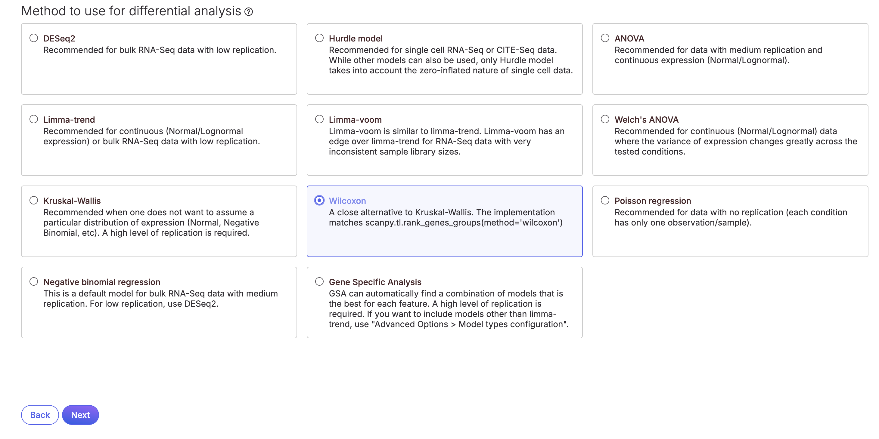
Powerful statistical analysis methods help identify differential expression patterns in the dataset. These can take into account a wide variety of data types and experimental designs. For differential expression analysis of spatial data we have implemented Wilcoxon. A nonparametric statistical hypothesis test that compares two groups and does not assume a normal distribution. Our implementation closely matches Scanpy's scanpy.tl.rank\_genes\_groups when using method='wilcoxon'.

To ensure meaningful results from the differential expression analysis, it's important to strike a balance between filtering the input data and configuring the filtering options within the analysis node. Overly stringent filters may result in no features passing the criteria, triggering a warning and halting the analysis. Conversely, minimal filtering may allow too many features, which can significantly increase processing time and require multiple testing corrections, potentially affecting statistical power.

**Running Wilcoxon**

We recommend normalizing you data prior to running *Wilcoxon*, but it can be invoked on any counts data node.

* Click the counts data node
* Click the **Differential analysis** section in the toolbox
* Click **Wilcoxon**
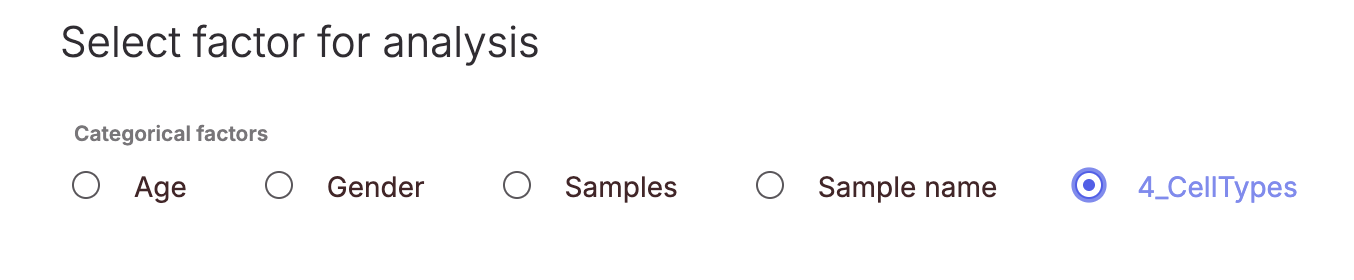
* Select the attribute to include in the statistical test , and click **Next**

<figure><img src="/files/K3gKStJhAYHl9ZU3en3w" alt=""><figcaption><p>Differential expression analysis method selection page.</p></figcaption></figure>

<figure><img src="/files/NUhVPFqsiPHf9ax7d1GJ" alt="" width="563"><figcaption><p>Attribute selection page.</p></figcaption></figure>

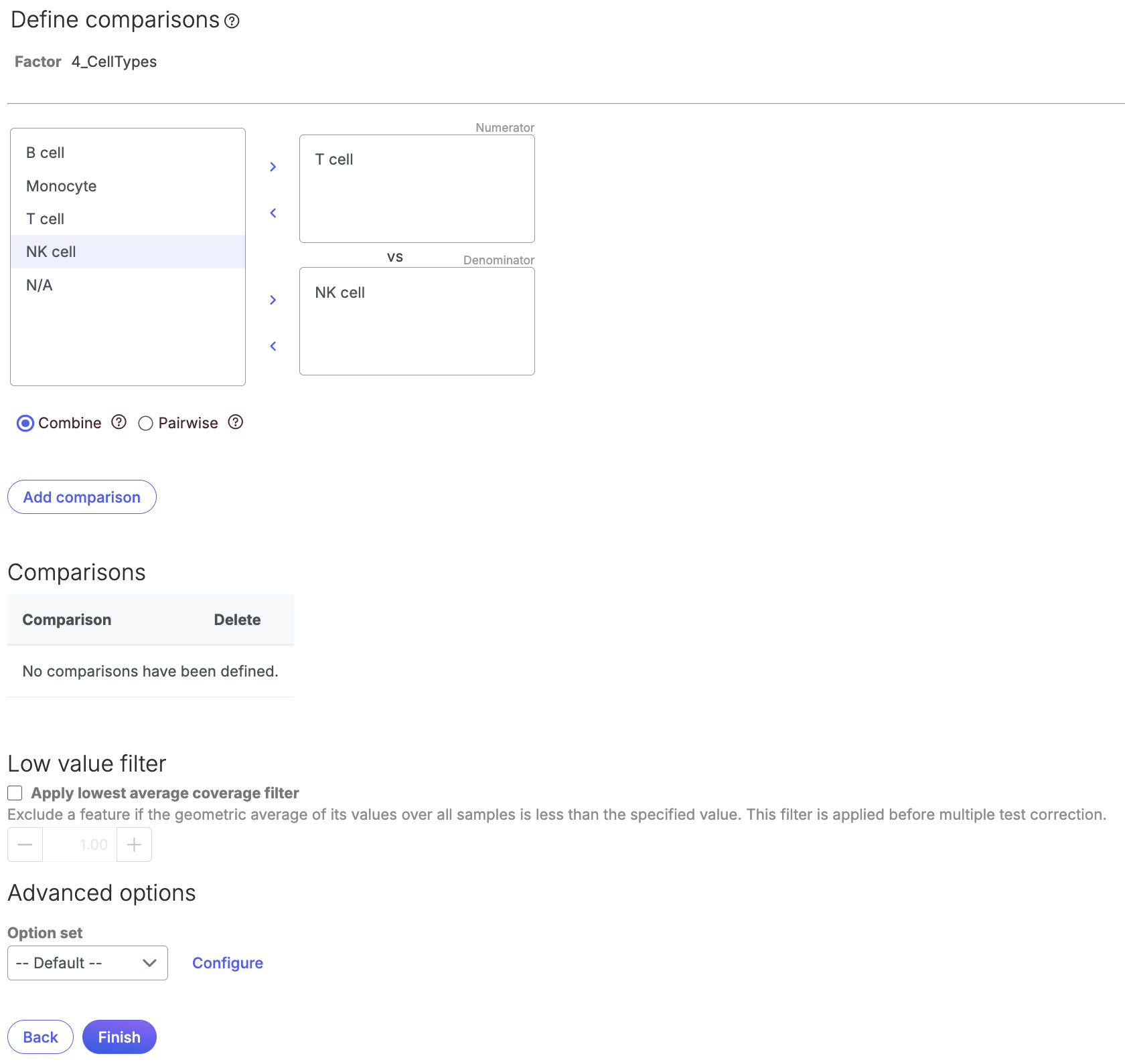
* Define the comparisons by dragging and dropping each group in the *Denominator* and *Numerator* boxes and click **Add comparison**

<figure><img src="/files/gS3bBdoOksb9RMxG9ke1" alt=""><figcaption><p>Comparison setup page.</p></figcaption></figure>

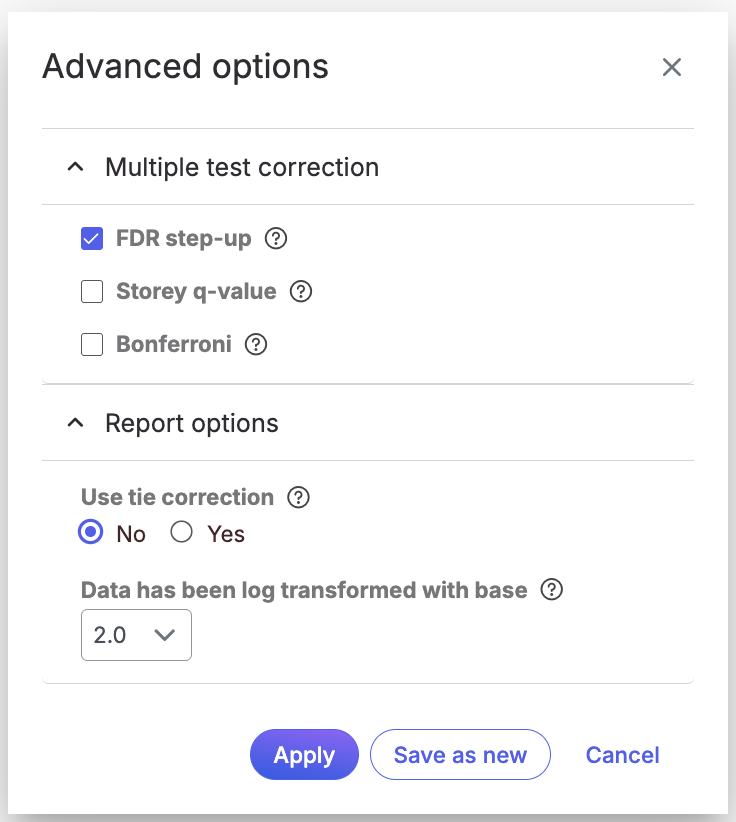
If the data has not been filtered upstream the **Low value filter** box will be checked by default. You can edit the filtering value and any of the **Advanced options** as needed. Click **Finish** to run the task.

<div data-full-width="true"><figure><img src="/files/OccfNWegZwo1L2HeAWTE" alt="" width="368"><figcaption><p>Advanced options menu</p></figcaption></figure></div>

### Wilcoxon task report

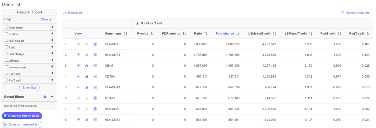
The Wilcoxon task produces a Feature list task node including these default report table parameters:

* Available feature information which may include Gene name, Gene ID and Transcript ID is displayed. Click the **View** options .... for more feature information
* The gene list table is sorted by the first p-value column
* The contrast outputs include P-value, FDR step up, Ratio and Fold change. Fold change is in linear scale. LSmean of each group in the comparison is in linear scale
* Clicking on the Optional columns link on the top-left corner of the table, displays extra information in the table when selected
* The volcano plot icon (![](https://help.partek.illumina.com/~gitbook/image?url=https%3A%2F%2F1384254481-files.gitbook.io%2F%7E%2Ffiles%2Fv0%2Fb%2Fgitbook-x-prod.appspot.com%2Fo%2Fspaces%252FJVEESmJAPppJ3ijFq5aR%252Fuploads%252Fgit-blob-578fb9619b29547466f026e1a653cbd219cede23%252Fvolcano_icon_gray.png%3Falt%3Dmedia\&width=40\&dpr=4\&quality=100\&sign=a626b8c6\&sv=2)) to the left of the Contrast title, displays the volcano plot for the chosen contrast in the Data Viewer.

<figure><img src="/files/7yQZp9E0ToZby4LFasRZ" alt=""><figcaption><p>Use the filter menu on the left to filter the reported features</p></figcaption></figure>

#### Filter the results

Filter the results using the feature list filter panel on the left of the table. Note that if more than one contrast has been included in the model, *All contrasts* or *Per contrast* options are provided.

* Click on the **black triangle** ( ![](https://help.partek.illumina.com/~gitbook/image?url=https%3A%2F%2F1384254481-files.gitbook.io%2F%7E%2Ffiles%2Fv0%2Fb%2Fgitbook-x-prod.appspot.com%2Fo%2Fspaces%252FJVEESmJAPppJ3ijFq5aR%252Fuploads%252Fgit-blob-4e879765e60ac81901020cd77deb18648802859c%252Farrow_down_icon_collapse_triangle_gray.png%3Falt%3Dmedia\&width=300\&dpr=4\&quality=100\&sign=3329f0fc\&sv=2) ) to collapse and expand the panel sections to customize the filter
* Select the **check box** of the field and specify the cutoff by typing directly or using the slider
* Press **Enter** to apply. After the filter has been applied, the total number of included features will be updated on the top of the panel (*Results*)

Use the buttons below the panel to **Generate a filtered node** on the analyses pipeline or **Save as a managed list**.

Generated filtered nodes can be used to run additional tasks in the Analyses pipeline such as generated a [heatmap and bubble map with hierarchical clustering](https://help.partek.illumina.com/partek-flow/user-manual/task-menu/exploratory-analysis/hierarchical-clustering) or performing [biological interpretation](https://help.partek.illumina.com/partek-flow/user-manual/task-menu/biological-interpretation/gene-set-enrichment).

## Marker Gene Identification

Compute biomarkers task is available as an independent task under Statistics in toolbox. It is also added as an option in the Clustering task dialogue.

The current implementation leverages the Scanpy 'rank\_genes\_groups' function, using the 'wilcoxon' method.

The task can be run on any counts node. If run from a non-normalised data node, the data will be normalised (scanpy.pp.normalize\_total) and logged (scanpy.pp.log1p). When run from the 'Statistics' menu as an independent task, follow the steps below:

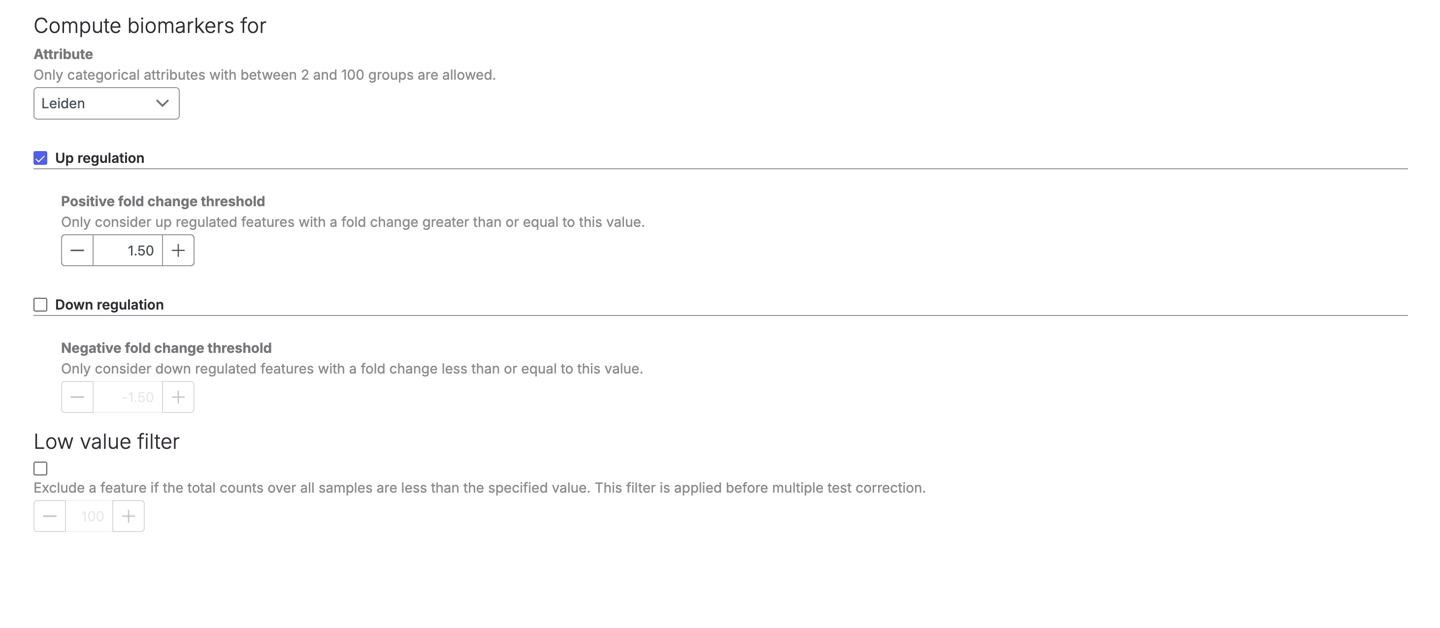
* Select the **Attribute** from the drop-down menu
* Select whether to compute Up or Down regulated genes, or both, using the **check boxes**
* If no filtering was applied to the node selected for the analysis, the 'Low value filter' option will be automatically selected
* Click **Finish** to run the task

<figure><img src="/files/ABPpPonWiods2E7QqwaI" alt=""><figcaption><p>Compute biomarkers setup page</p></figcaption></figure>

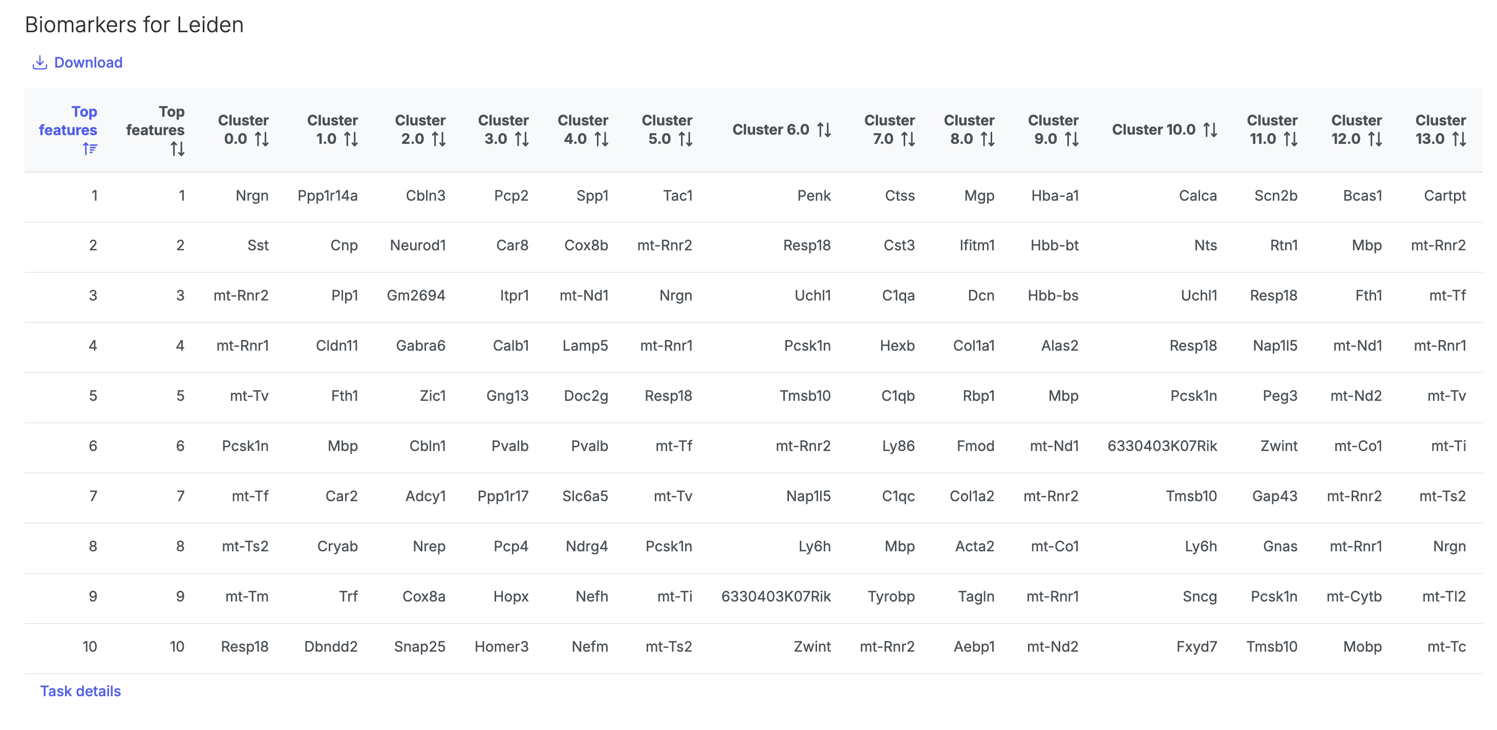
The task will generate a biomarkers table listing significant (adjusted p-value < 0.05, LFC as set in the task) genes for each category in the selected attribute:

<figure><img src="/files/caCKjylrKNvuiAH29m4p" alt=""><figcaption><p>Table of results produced by the Compute biomarkers task.</p></figcaption></figure>

## Cell Typing

Cell typing (classification) can be done manually and automatically.

### Manual classification

Manual and criteria selections are used to classify cells in the Data Viewer.

Feature lists can be added and used to help with manual classification. <https://help.connected.illumina.com/icm/analyses/analysis-functionality/settings/lists>

### Automatic classification

ScType is "a fully-automated and ultra-fast cell-type identification based solely on a given scRNA-seq data, along with a comprehensive cell marker database as background information."\[4]. It allows accurate cell typing in scRNAseq and spatial transcriptome data \[5].

The task can be called from any non-normalised counts node, in the *Classification* menu on the right.

* Click on the Counts node.
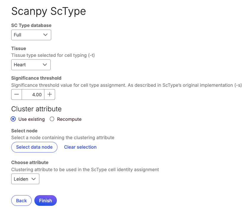
* Click on *Classification> Scanpy ScType* in the toolbox.
* Select you **marker database** from the drop down menu, or create a new one (see below).
* Select the significance threshold. This number indicates the fraction of cells, higher numbers indicate a less strict significance threshold (see paper for method details).
* Choose the tissue type from the drop-down.
* If using an existing attribute for the classification, select the node and the attribute from the drop-down, by default a Leiden clustering node will be selected (if it exists).
* You can select *Recompute* if you wish to run Leiden as a part of this task, and edit the resolution parameter as needed.
* Click **Finish** to run the task.

<figure><img src="/files/sdvUCiZfJx2xL0AV0Nct" alt="" width="563"><figcaption></figcaption></figure>

The task outputs an annotation for each cell in the dataset. If a cell does not pass the significance threshold it will be classified as "Unknown". The annotation is saved as 'sctype\_classification', and is available from the node. You can use *Annotation/Metadata>Publish cell attributes to project* in the toolbox to make the attribute available at the Analysis level.

### Select database

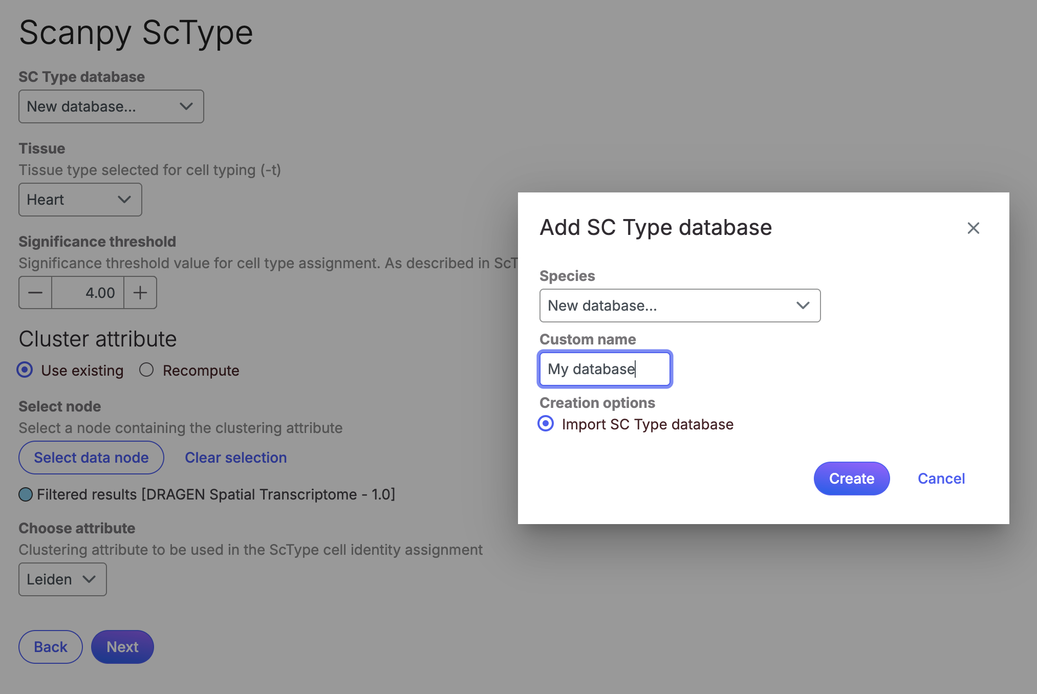
ScType will use the curated marker database for human and mouse found here: <https://sctype.app/database.php>. Users can provide their own marker database, formatted as the original, by selecting *New database* from the **ScType database** dropdown:

* In the **SC Type database** dropdown, select *New database.*
* Give the database a custom name (eg. "My database"), and click **Create**.
* Navigate to the correct file and select it (valid formats are .tsv, .txt, .csv).

<figure><img src="/files/BMRe7GnA01CzmV0qpjqG" alt=""><figcaption></figcaption></figure>

## Cell-cell communication

### CellphoneDB

CellPhoneDB addresses the challenges of studying cell-cell communication in scRNA-seq and spatial data. It allows researchers to move beyond just measuring gene expression and delve into the complicated cellular communication world. By analyzing the scRNA-seq or spatial data through the lens of CellPhoneDB, researchers can identify potential signaling pathways and communication networks between different cell types within the sample. Connected Multiomics wrapped the statistical analysis pipeline (method 2) from CellPhoneDB v5 \[6]\[7] for this purpose.

### How to use CellPhoneDB <a href="#how-to-use-cellphonedb" id="how-to-use-cellphonedb"></a>

Invoke the **CellPhoneDB** task from a normalized counts data node using the *Exploratory* *analysis* section. We recommend running CellPhoneDB on the log normalized data directly. To run **CellPhoneDB** task:

* Click a **Normalized** **counts** data node
* Click the **Exploratory analysis** section in the toolbox
* Click **CellPhoneDB**

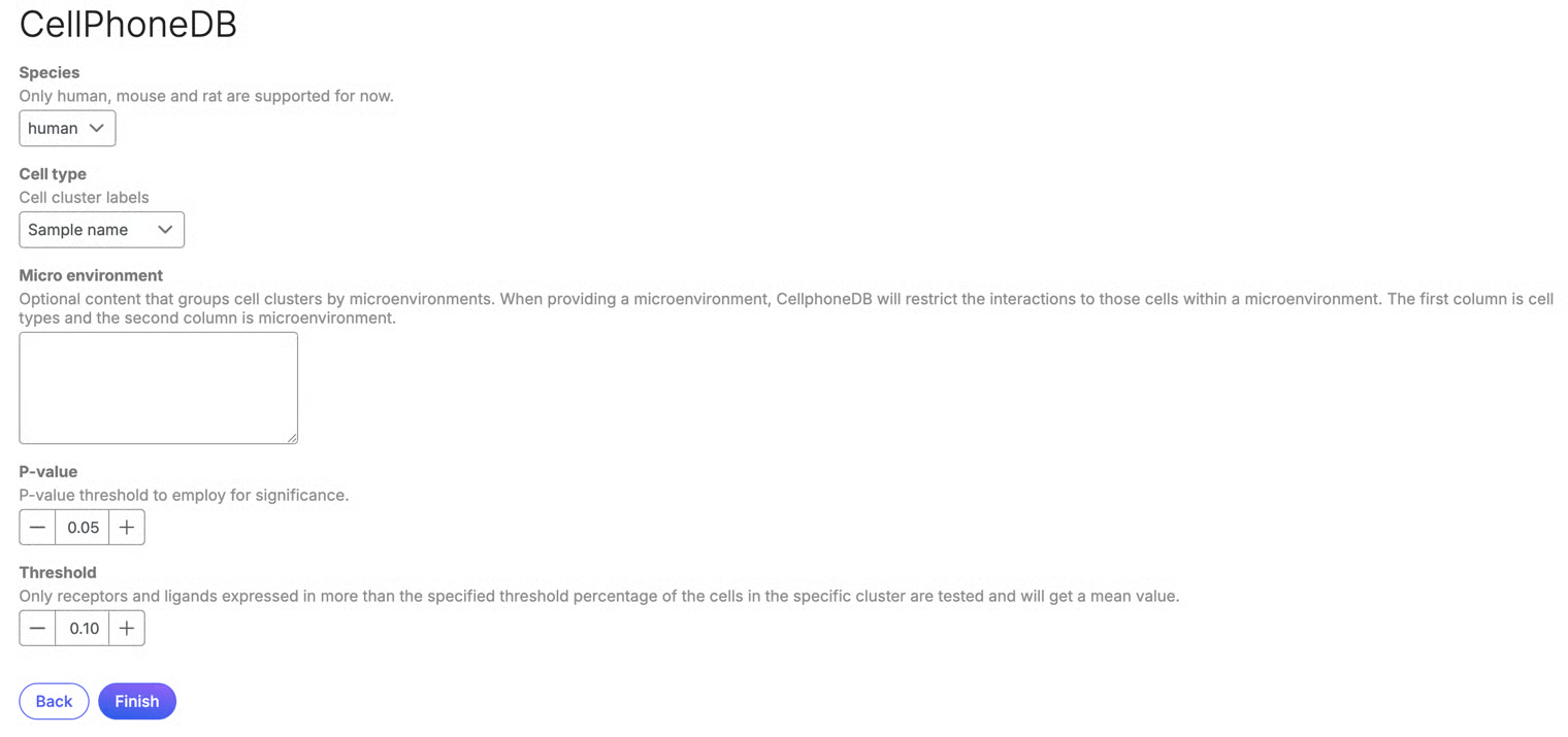
<figure><img src="/files/OCuqhxe6sdWrNowxN3V3" alt=""><figcaption></figcaption></figure>

**Species**

Currently human, mouse and rat are supported. Select the species of the data from the drop-down list.

**Cell type**

Select the attribute from the drop down. Any categorical attribute associated with the data can be selected, though typically the task is performed on cell typing results.

**Micro environment**

The micro environment file is typically used when analyzing spatial data (see the tool's [documentation](https://cellphonedb.readthedocs.io/en/latest/RESULTS-DOCUMENTATION.html#microenvironment-file)), and it is optional. The micro environment information can be added to the task using the text box in the task. This can be simply copy-pasted from a micro environment file, a .txt with two columns indicating which cell type (1st column) is in which spatial microenvironment (end column).

**P-value**

Specify the p-value cutoff to employ for significance

**Threshold**

By default, the value of 0.10 will be used as threshold to select which cells are used for the analysis in the cluster. However, the number could be adjusted manually or typed in directly.

Click the **Finish** button if you want to run the task as default.

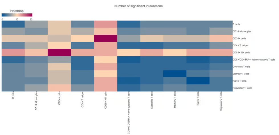
Double click the CellPhoneDB result data node will open the task report in Data Viewer. It is a heatmap that summarizes how many significant interactions identified in the cell type pairs.

<figure><img src="/files/zaJrPN4zkO1HazAKmQRZ" alt=""><figcaption></figcaption></figure>

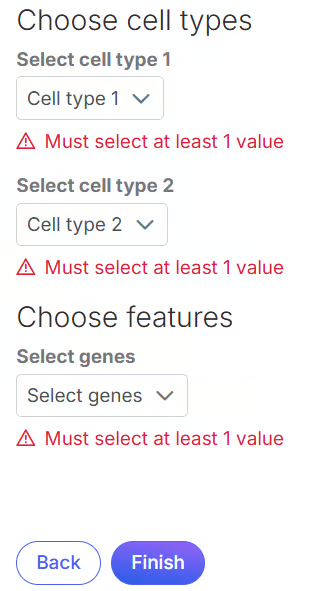
To explore more, the task of **Explore CellPhoneDB results** under *Exploratory analysis* on the pop-up menu. It allows you to focus on specific cell type pairs and genes of interest. Genes of interest are data dependent and usually come from the published results of similar studies or the differential gene analysis between different conditions (eg, cancer patient vs healthy controls). Once set up, click the **Finish** button to submit the job.

<div align="left"><figure><img src="/files/mucLDSpWOesNRSoSVbKJ" alt="" width="236"><figcaption></figcaption></figure></div>

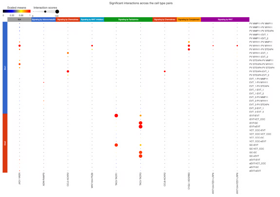
Double click the Output matrix data node will open the task report in Data Viewer. It is another variant of heatmap that displays how genes of your interest interact in the defined cell type pairs.

<figure><img src="/files/BDgxOQaE0tTsYCgbGiHl" alt=""><figcaption></figcaption></figure>

The exampled plot also indicates the data are from two environments. For instructions on setting up the Micro environment file for your spatial study. CellPhoneDB analysis classifies signaling pathways for genes of interest. These classifications are then used to annotate the heatmap within the task report.

### Why are the values of clusterA-clusterB different to the values of clusterB-clusterA? <a href="#why-are-the-values-of-clustera-clusterb-different-to-the-values-of-clusterb-clustera" id="why-are-the-values-of-clustera-clusterb-different-to-the-values-of-clusterb-clustera"></a>

It is important to note that the interactions are not symmetric. The authors state that, "Partner A expression is considered for the first cluster/cell type (clusterA), and partner B expression is considered on the second cluster/cell type (clusterB). Thus, *IL12-IL12 receptor* for clusterA-clusterB (i.e. the receptor is in clusterB) is not the same as *IL-12-IL-12 receptor* for clusterB-clusterA (i.e. the receptor is in clusterA), and will have different values." \[8]\[9]

### Where do the interactions come from? <a href="#where-do-the-interactions-come-from" id="where-do-the-interactions-come-from"></a>

The interactions come from the CellphoneDB database. It is manually curated repository using reviewed molecular interactions with demonstrated evidence for a role in cellular communication. \[10]

## References

\[1] McInnes L and Healy J, UMAP: Uniform Manifold Approximation and Projection for Dimension Reduction, ArXiv, 2018, e-prints 1802.03426.

\[2] L.J.P. van der Maaten and G.E. Hinton. Visualizing High-Dimensional Data Using t-SNE. Journal of Machine Learning Research 9(Nov):2579-2605, 2008.

\[3] Becht E, McInnes L, Healy J, Dutertre A-C, Kwok I, Guan Ng L, Ginhoux F, and Newell E, Dimensionality reduction for visualizing single-cell data using UMAP, Nature Biotechnology, 2019, 37, 38-44.

\[4] Ianevski, A., Giri, A. K., & Aittokallio, T. (2022). Fully-automated and ultra-fast cell-type identification using specific marker combinations from single-cell transcriptomic data. Nature communications, 13(1), 1246.

\[5] Nader, K., Tasci, M., Ianevski, A., Erickson, A., Verschuren, E. W., Aittokallio, T., & Miihkinen, M. (2024). ScType enables fast and accurate cell type identification from spatial transcriptomics data. Bioinformatics, 40(7), btae426.

\[6] *Troule, etc (2023)*. CellPhoneDB v5: Inferring cell-cell communication from single cell multiomics data. <https://arxiv.org/pdf/2311.04567.pdf>​

​\[7] <https://github.com/ventolab/CellphoneDB>​

​\[8] <https://github.com/ventolab/CellphoneDB/blob/master/docs/RESULTS-DOCUMENTATION.md>​

​\[9] <https://cellphonedb.readthedocs.io/en/latest/RESULTS-DOCUMENTATION.html#why-values-of-clustera-clusterb-are-different-to-the-values-of-clusterb-clustera>​

\[10] ​<https://github.com/ventolab/cellphonedb-data>​


---

# Agent Instructions
This documentation is published with GitBook. GitBook is the documentation platform designed so that both humans and AI agents can read, navigate, and reason over technical content effectively. Learn more at gitbook.com.

## Querying This Documentation
If you need additional information that is not directly available in this page, you can query the documentation dynamically by asking a question.

Perform an HTTP GET request on the current page URL with the `ask` query parameter, and the optional `goal` query parameter:

```
GET https://help.connected.illumina.com/dragen-stratamap/illumina-connected-multiomics/spatial-analysis/additional-analysis.md?ask=<question>&goal=<endgoal>
```

`ask` is the immediate question: it should be specific, self-contained, and written in natural language.
`goal` is optional and describes the broader end goal you are ultimately trying to accomplish on behalf of the user. GitBook uses it to tailor the answer towards what is most useful for that goal.

The response will contain a direct answer to the question and relevant excerpts and sources from the documentation.

Use this mechanism when the answer is not explicitly present in the current page, you need clarification or additional context, or you want to retrieve related documentation sections.