For the complete documentation index, see llms.txt. This page is also available as Markdown.

Perturb-seq

Illumina Connected Multiomics

Illumina Connected Multiomics (ICM) is available for further tertiary analysis of Illumina Single Cell Transcriptomics Perturb-seq data and other multiomic data.

Getting Started

Refer to the following links to the ICM user guide to get started with ICM:

Demo Data

Demo data that can be used to follow along with this walkthrough is found in the Connected Multiomics Demo Data repository and can be found under Single cell > Perturb-seq.

Each sample will need the following files as input (when specifying sample1 as the sample id):

  • sample1.scRNA.filtered.matrix.mtx.gz

  • sample1.scRNA.filtered.barcodes.tsv.gz

  • sample1.scRNA.filtered.features.tsv.gz

  • sample1.scRNA.feature_barcode_reference.csv

  • sample1.scRNA.positive_cell_guide_assignments.csv

This data is one sample consisting of Human A549 cell line. As determine by DRAGEN, each cell barcode present is a positive cell assignment (cells below a certain threshold are filtered out). The num_transcripts (number of transcripts) represents coverage of the guide as read counts.

Default Single Cell Perturb-seq Analysis

The default Perturb-seq analysis runs a pre-defined pipeline on each sample and presents analysis results in visualizations in a Data viewer.

Creating a Default Analysis

After adding data to a study, follow the following steps to create a Default analysis.

  • Select the samples to include in the analysis

  • Click on + Create analysis

Select samples and Create analysis
  • In the pop-up window, provide a name for the analysis

  • select Default: Illumina Single Cell Transcriptomics Perturb-seq from the dropdown as the Analysis type

  • click on the Run Analysis button

Define Default or Custom analysis

View Default Analysis Results

The analysis status will change to Complete when the analysis has finished.

  • Click on the analysis tile to open results

The analysis opens to the analysis task graph.

The task graph shows the analysis pipeline

The first task run on the imported data, Split by feature type, is to split the data into different features: CRISPR Direct Capture (gRNAs) and Gene Expression. This is because having gRNAs included in standard analyses for both clustering and differential expression can lead to unexpected clustering results. The remainder of the pipeline follows the standard scRNA-seq workflow. Additional details for each task are available via the Single Cell walkthrough.

View Summary report

  • Double-click the Summary report to open a Data viewer session.

Double-click to view the Summary report

The Summary report shows the Gene expression tab and CRISPR Direct Capture tab from the Perturb-seq samples; these can be toggled at the bottom of the data viewer session.

Gene expression tab

The Gene expression tab consists of one UMAP colored by cluster IDs, a biomarker table, a cell composition pie chart and the distributions of Total count and Expressed genes within different clusters.

Gene expression data from the Perturb-seq samples
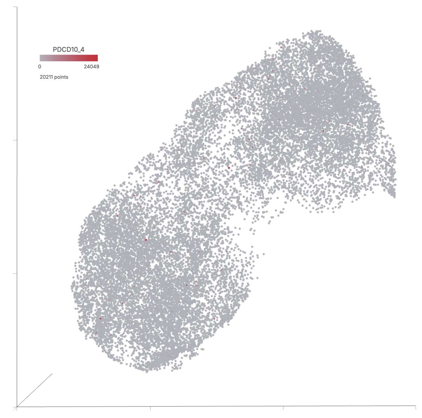
The plots can be configured by selecting the Configure option from the toolbox on the left within each plot. Here is one example that converts the above UMAP to a feature plot by recoloring single cells with a ‘feature’: one of the gRNAs (PDCD10_4). In the feature plot, all cells in red carry the perturbation of the gRNA, while all the non-perturbation cells are in grey for this specific guide.

CRISPR Direct Capture tab

The CRISPR Direct Capture tab consists of the frequency of the total number of features (guides) in the cells as well as the frequency of each of the top 10 features with highest sum.

CRISPR Direct Capture data from the Perturb-seq samples

Additional information for custom analysis

Example pipeline

A typical custom pipeline includes both the gene expression analysis and CRISPR Direct capture analysis.

Example Custom Perturb-seq analysis

Single cell QA/QC task

It is optional to filter only high quality cells based on the total count, detected features, % mitochondria, and % ribosomal counts.

  • Select the Single cell QA/QC task, under QA/QC in the task menu

    • This results in the Filtered cells results node

Filter cells (observations)

It is optional to filter the cells. In the next step (shown on the pipeline as the Filter observations task), we will filter the cells by metadata to include cells with a number of features = 1.0. We chose to do this because this will filter our the cells to include 1 guide per cell and remove the cells with more than 1 guide or cells with no guides to limit combinatorial effects. There are cases where you might keep multi-guide cells and this should be based on your experimental design and research question.

  • From the Filtered cells node, open the Filter cells task under Filtering in the task menu

  • Filter by Metadata to Include the num_features = 1.0

  • Click Finish

num_features is CRISPR metadata. We are not filtering gene expression data in this step

This results in a counts node filtered to cells including 1.0 number of features (CRISPR guides).

Counts node with cells including 1.0 CRISPR feature guide per cell

Split by feature type

Split by feature type is used to split and analyze the CRISPR Direct Capture and Gene expression features independently.

  • Select the Split by feature type task under Pre-analysis tools in the task menu

This results in a node containing the CRISPR Direct Capture features and node containing the Gene expression features.

Split by feature type to analyze the CRISPR and Gene expression data

Create the CRISPR Direct Feature Data viewer session

  • Click the Data viewer tab

Click the Data viewer tab
  • Click Create new view

Create new Data Viewer session
  • Click Setup

  • + New plot

Add new plot to Data viewer session
  • Choose Bar chart as the plot type

  • Select Filtered Features node as the data to plot

  • Choose num_features as the data attribute

  • Modify the Axes configurations as shown below to match the settings from the CRISPR Direct Feature Data viewer session tab

Modify Axes settings to change the visualization
  • Add another bar chart but this time choose ATM/design_3 as the content data to plot

  • Click Add

  • Modify the Axes settings to match below

  • Duplicate the plot 9 times

Duplicate the plot
  • Change the Axes content data to the other top features.

Ctrl+Click and drag to resize views without snapping. Click the Save button to Save over an existing session or Save As to save a new Data viewer session.

Resize views and Save the Data viewer session

Select cells by criteria

Selection > Select & Filter can be used to select cells with specific targets. Our input data from DRAGEN contains a Feature call label and Target gene name. Either of these can be used to select cells matching the criteria.

  • Select the criteria and enter the name of interest to select the cells

These cells could be labeled and classified using Selection > Classify.

Classify the Non-Targeting control and Perturbed cells population

Depending on your experimental design and research question there can be different populations of cells that could be used as controls. This could be non-targeting controls, cells with no detected guide, or all cells carrying guides other than the guide of interest. In this data, we have already filtered to the cells containing one CRISPR guide, so we will not use cells with no detected guide as the control. Below we will demonstrate classifying the non-targeting controls and perturbed cell populations.

  • Classify the selection as Perturbed cells

Use the Apply classifications button to make the cell-level attribute (Classification) available from all data nodes within the analysis, including for use with differential analysis.

Last updated

Was this helpful?